
Copyright © "Six Meter International Radio Klub" · All Rights reserved

This section is designed to help new six meter operators get the best out of their equipment, band openings, and explain a few of the mysteries of the "Magic Band".
First, what is six meters? Simply put six meters is the frequency band allotted to amateur radio operators starting at 50.0 Megahertz and ending at 54.0 Megahertz. This band encompasses all modes of communications but is broken down into segments so that there is minimal interference between the different modes and and interests. The band plan for the United States (IARU Region 2) was promulgated by the ARRL and is the accepted norm. IARU Region 1 and IARU Region 3 have seperate but similar plans.
U.S. Band Plan
50.0-50.1 CW, beacons, CW Mode only under FCC Rules
50.060-50.080 beacon subband required to be used under FCC Rules by US licensed stations
50.1-50.3 SSB, CW
50.10-50.125 DX window
50.125 Domestic calling frequency
50.25 - 50.28 WSJT
50. 290 US PSK calling frequency
50.3-50.6 All modes
50.6-50.8 Nonvoice communications
50.62 Packet calling
50.8-51.0 Radio remote control (20-kHz channels)
51.0-51.1 Pacific DX window
51.12-51.48 Repeater inputs (19 channels)
51.12-51.18 Digital repeater inputs
51.62-51.98 Repeater outputs (19 channels)
51.62-51.68 Digital repeater outputs
52.0-52.48 Repeater inputs (except as noted; 23 channels)
52.02, 52.04 FM simplex
52.2 TEST PAIR (input)
52.5-52.98 Repeater output (except as noted; 23 channels)
52.525 Primary FM simplex
52.54 Secondary FM simplex
52.7 TEST PAIR (output)
53.0-53.48 Repeater inputs (except as noted; 19 channels)
53.0 Remote base FM simplex
53.02 Simplex
53.1, 53.2, 53.3, 53.4 Radio remote control
53.5-53.98 Repeater outputs (except as noted; 19 channels)
53.5, 53.6, 53.7, 53.8 Radio remote control
53.52, 53.9 Simplex
As you can see the six meter band is quite large and accommodates many different modes and interests. The two major modes of interest are SSB telephony and CW so we will concern ourselves with just those two modes. SSB is used from 50.100 to 50.300 MHz. This is broken down into 2 seperate areas, 50.100 to 50.125 MHz is considered the DX Window with 50.110 MHz the DX Calling Frequency. Domestic qso's should NEVER occur in the DX Window. What are domestic qso's? Basically any qso between U.S. stations (lower 48 states) or U.S. and lower tier VE stations. There is plenty of room for these contacts above 50.125 MHz, the domestic calling frequency. Alaska, KL7 and Hawaii, KH6 are considered DX stations.
Domestic Calling Frequency, 50.125 MHz
This is the frequency where you can usually drum up a qso if the band is open. Remember, this is a calling frequency and once you have established contact with someone please move (qsy) up the band. Someone else may want to call. During contests it is not considered good practice to monopolize the calling frequency. Stations will hear you wherever you are.
Beacons, Digital Modes and CW
Voice communications may not be used below 50.100 MHz as that is reserved for CW and beacons. You will normally find domestic CW stations between 50.080 and 50.100 MHz while the beacons are below 50.080 MHz. This is not to say that CW is confined there as it may used throughout the entire band. PSK has an informal calling frequency of 50.290 MHz in the United States. WSJT signals are usually found between 50.250 and 50.280 MHz in the U. S. WA5UFH has a great site that explains WSJT and operating procedures. The considerate operator will always operate within the parameters of the band plan. Now that we know where to operate we will discuss how to operate.
Getting started
Most new operators lose their "mike fright" soon after their first contact. Six meter operators are some of the best in the world because it is a challenging band. The best way to get started is to call a CQ. Pick a frequency or go to the calling frequency, 50.125 MHz, check to see if it is busy and if it is not go ahead and put out your CQ. Do not use long CQ's. If the band is open it will just annoy other operators and if it isn't it just won't matter. Several short CQ's are better than one long one. The best way to call CQ is to say "CQ CQ CQ this is (your call, your call), over." To answer a CQ give the calling stations callsign followed by "this is (your callsign), over." Example: AA5XE this is W5OZI, over. After the contact is initiated you may talk about whatever your heart desires. Just remember to identify your station at least once every ten minutes and at the end. There are a lot of stations that are only interested in your grid and a signal report or just making a very short contact. One of the signs of a new operator is to use "personal" instead of "name." This usually marks someone as brand new. Remember, it is always best to be clear and concise. Use the ITU phonetic alphabet as it makes understanding universal. Cute phonetics can be very confusing, especially under marginal band conditions or when operating with a DX station. The best operators are the ones that are clear, concise, polite, and follow the band plan. A good discussion of this is found at the United Kingdom Six Meter Group site, Voluntary Operating Code of Practice for 6m Operators and is generally applicable to all operators.
Logs and QSL's
One should generally keep a record of their contacts. There are many good computer logging programs out there, many of them freeware, as well as paper logs. The ARRL sells logbooks cheaply. There is a keen interest among six meter operators to work as many grids as possible. If you make contacts, you will receive QSL cards wanting you to confirm the contact. The final courtesy of any qso is to qsl. This is why logging is important. There are many companies that make qsl cards or you can make your own. Some may be very fancy and expensive while others are bare bones. It makes no difference as long as the required information is present. A good qsl will have the name, address, callsign, and grid of the operator with the date, time in UTC, RST, and mode of operation and the callsign of the other station. A good idea is to include a self addressed, stamped envelope (SASE) along with your qsl request. Don't make the other operator bear your expense if it is you that wants HIS card. There are many variations on qslling. Some initiate a qsl for every contact while others only send qsl's for new grids or countries. However you want to do it is up to you. You should always answer every qsl received, though. You may be the rare contact to the other station. If you are in to DX you should keep a supply of envelopes on hand at your incoming qsl bureau. Bureaus are used to minimize the cost of postage and is a good way to save on qsl costs. The ARRL operates an outgoing qsl service for its members which is widely used.
Hardware
The main part of any station should be the antenna. Put up the best antenna you can afford. CW and SSB signals are generally horizontally polarized so you should consider a beam antenna. Vertical antennas will work for strong E skip but nowhere near as well as a horizontal yagi. An old maxim applies here, "Big antennas, high in the sky will always beat small ones low to the ground." Next comes the radio. Find what you like and can afford. Many start with used equipment. There are several places on the web where you can find used equipment. There are many radios out there now that make six meters an integral part of the radio. Some still prefer to use down converters with an existing HF rig but that is personal choice. What many people forget is that if you buy a $10,000 radio and connect a $2 antenna to it, you now have a two dollar radio. Install your system where you won't disturb your family nor they you when you are operating. The main idea here is to be comfortable. Make sure your equipment is grounded. It is always better to be safe than sorry. Unplug your antennas during your abscence and during lightning storms. You might consider purchasing insurance for your equipment. The ARRL has an insurance plan for a modest price that will insure your equipment and antennas.
Clusters and the Internet
One place you can find out lots of information on who is hearing who is a packet cluster. Packet clusters are now in reach of just about everyone. They are still on the packet frequencies and on the internet. There are many good dx clusters on the internet that cover the entire world. There is wealth of information to be had on the internet. Another good source of information is the 50 MHz Propagation Logger. The ON4KST's Chat pages is another good place to be. It gives information in real time. You do have to register and log in as a user. There is a SMIRK mailing list maintained by Al Waller, K3TKJ at www.qth.net . This is just one of many lists that he maintains. The SMIRK website offers a tremendous amount of information concerning six meters, from contest information to qsl information. The qsl info page has one of the most up to date databases of qsl information around, not just for six meters either. You can also find the latest information on six meter DXpeditions in the DX section. There are many good six meter links at the site.
PROPAGATION ON THE MAGIC BAND
By Robert Magnani K6QXY
6 meters is a very unique amateur band. Every mode of propagation known to exist can be found here. In fact, the 6 meter amateur band was actually an FCC compromise that recognized the importance of this block of frequencies. Originally the Commission was going to give amateurs a band between 44 and 48 mhz. Intense lobbying by the ARRL convinced the FCC there were enough unique propagation attractions to assign the 6 meter band to 50-54 mhz.
There are three major forms of propagation that can cause real excitement on the Magic Band.
F-Layer Propagation
Approximately every 11 years the sun explodes into violent solar storms. These solar storms produce sufficient amounts of radiation to excite the F-layer producing a very radio reflective surface. A smoothed sun spot number of at least 120 is needed for the M.U.F. (maximum useable frequency) to reach 50 mhz. When this occurs, 50 mhz. signals can be propagated to distances exceeding 10,000 miles!!!!
The height of the ionized F2 layer reflections produce single hop distances approaching 2,500 miles. With the sun rotating on its axis every 27-28 days, a sun spot or complex group of spots, will again face the earth and a particular series of events will often repeat itself every 27-28 days.
Transequitorial Propagations
One of the most exciting propagation modes is transequitorial propagation or TEP. TEP is really the scattering from ionospheric irregularities at very high altitudes. Actually TEP was discovered by amateurs during the late 1950s. They called the new mode Transequitorial Field Aligned Irregularities.
TEP forms across the Geomagnetic Equator, with stations ideally situated on a north south axis at equal distances either side of the Geomagnetic Equator. Occurring near the two solar equinoxes in March and September, TEP occurs in the late afternoon and early evening. There is a strong positive correlation with the solar cycle peak. M.U.F.s of TEP signals can often exceed 400 mhz. There is a strong correlation between the formation of TEP and auroral events. TEP signals often exhibit the same garbled characteristics as that of auroral scattered signals.
Sporadic E
One of the most misunderstood VHF propagations modes is Sporadic E. Sporadic E normally displays a major peak during the summer months of May through August, and then again with a minor peak in the winter months of November and December.
Sporadic E appears to be reflections from dense patches of ionization that form at E-layer heights. The height of the E-Layer reflections produce single hop distances on the order of 1,200 miles. One, two, three and even four hop sporadic E has occurred with distances exceeding 5,000 miles. Whether they are actually hops that touch the earth or Chordial Hops that just graze the earth or even cloud to cloud reflections is not clear. The actual cause of sporadic E is unknown. Theories include high altitude wind sheer and the generation of strong electron fields associated with high altitude thunder storms. Research now indicates that certain multi-hop Sporadic E paths, especially those that cross the Auroral E Zone and the Equitorial E Zone exhibit strong diurnal characteristics. These paths show a remarkable consistency in time of day, month and year repeatability.
There does not seem to be any correlation with the 11 year solar cycle, but data seems to suggest a 5-7 year cycle with a 5-7 day underlying cycle.
Other forms of propagation on the Magic Band include meteor scatter, aurora and Auroral Es plus the various scatter modes. All of these in combinations with the above mentioned major modes contribute to exciting times on 6 meters.
A must reading for all Magic Band enthusiasts is the ARRL publication Beyond Line of Sight by Emil Pocock W3EP. Emil brings together articles and papers on VHF propagation from the pages of QST. Another fine source of 6 meter propagation data can be found on Bob Mobiles (K1SIX) site .
Where Do the K and A Indices Come From?
Carl Luetzelschwab K9LA
(This article appeared in K9LA's monthly Propagation column in the October 2003 issue of WorldRadio. Reprinted by permission.)
The K and A indices are readily available parameters (for example, they're given at 18 minutes past the hour on WWV) that can give us an indication of how the high latitude ionosphere might be affecting propagation. Let's take a look where the K and A indices come from to hopefully gain a better understanding of these important propagation parameters.
It all starts with the K index. The K index is a 3-hour measurement of the variation of the Earth's magnetic field relativeto quiet day conditions. The K index is determined from the data taken by a magnetometer, which measures the variation of the magnetic field in nanoTeslas (nT). Table 1 shows the nT range versus the K index for the mid latitude Boulder, Colorado, USA magnetometer.
If we plot nT (using mid range values of nT) versus K, we get the plot of Figure 1.

C
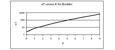
Table 1
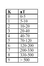
Figure 1
Note that nT is plotted on a logarithmic scale and that the curve is almost a straight line. Since it isn't exactly a straight line, the K index is said to be quasi-logarithmic.
Before moving on, an important comment is in order. Each station has its own scale of nT versus K. This is done to try to make the K index from each station represent the same level of disturbance. For a given disturbance, the variation in the Earth's magnetic field will be greatest at the high latitudes. Thus at the high latitude College (Alaska) station, a K index of 9 is a variation greater than 2500 nT. At the low latitude Kuyper (Sumatra) station, a K index of 9 is a variation greater than 300 nT. Compare these nT values with the mid latitude Boulder nT value of K=9 in Table 1.
Now lets look at a magnetometer record (which is called a magnetogram) to see how the K index is determined. Figure 2 is a snapshot of the magnetogram from Boulder on April 16, 2003 (thanks to Dr. Christopher Balch at NOAA/SEC).
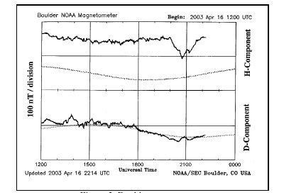
Figure 2 - Boulder Magnetogram
The solid line at the top of the plot is the variation of the H-Component (vector horizontal component) of the magnetic field. The dotted line about one vertical division below this solid line is the quiet day curve for the H-Component.
The solid line at the bottom of the plot is the variation of the D-Component (magnetic declination) of the magnetic field. The dotted line running almost concurrent with this solid line is the quiet day curve for the D-Component.
The K index for any three hour period is first found by finding the maximum positive and negative deviations for both components relative to their respectiv quiet day curves. Next these are added together for each component to determine the maximum fluctuation of each component. The component with the largest fluctuation is used to determine the K index. In the 1200-1500 UTC period of Figure 2, for example, the D-Component exhibits the maximum deviation from the quiet day curve. This is easiest seen by mentally overlaying the H-Component quiet day curve on the H-Component data, and noting the H-Component varies less about its quiet day curve than the D-Component.
The maximum positive deviation for the D-Component is +35 nT around 1350 UTC. The maximum negative deviation is -10 nT around 1440 UTC. The maximum fluctuation is therefore (+35nT) - (-10nT) = 45 nT. Going to Table 1 says the K index for this period is 4, which is what Boulder reported. In a similar manner, the K indices for the other seven 3- hour time periods can be determined. Note that the magnetometer only measures the deviation from a quiet day curve, not an absolute value.
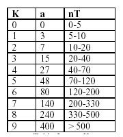
Table 2 - A vs K
If we now plot nT versus the a index we get Figure 3.
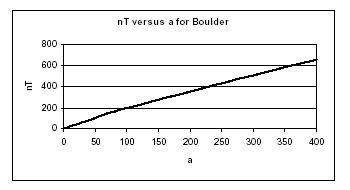
Figure 3
Note that nT is now plotted on a linear scale and that the resulting curve is for all intents and purposes a straight line. Thus the 3-hour a index (and the subsequent A index) is said to be linear.
Now we can simply add the 8 3-hour a indices, divide by 8, and come up with a daily average - which is the A index. We can also do this for many worldwide stations and come up with the daily average planetary A index, Ap. In a like manner, we can use many worldwide stations to come up with the 3-hour planetary K index, Kp.
Ok, now we know where K and A come from. But how do they tie to HF and VHF propagation conditions? In general, as the K and A indices become elevated:
1. The high latitude E region ionization can increase significantly (VHF'ers like this)
2. Increased D region absorption in and near the auroral oval (not good)
3. Usually the F region ionization at mid and high latitudes decreases (not good)
4. Sometimes, depending on how the geomagnetic storm evolves, the F region ionization at low and mid latitudes increases (this can be good)
The extent to which the above events occur on a specific path is hard to pin down. It depends on the geomagnetic storm itself, the geomagnetic latitude along the path, the level of solar activity, the season, and the local time along the path. Both W6ELProp and ICEPAC (the derivative of IONCAP that incorporates a high latitude ionosphere model) allow input of the K index to make a broad assessment of the impact of an active geomagnetic field.
One last 'problem' should be mentioned. The K index and thus the a and A indices are measurements of currents flowing at E region altitudes. Thus they don't really give us any indication of what's going on at F region altitudes. Addtionally, since the A index is the average of eight K indices, a spike in one or two of the eight 3-hour K indices may not show up very much in the daily average A index, even though the spike affected the ionosphere. So the A index could be encouraging, but it may not indicate the effects of a short- term event. A good example of this 'problem' is what happened to 10M in the CQ WPX contest in 2002. See the March 2003 issue of CQ for details of this.
There you have it. You should now have a good understanding of how the K and A indices are determined.
Helpful Propagation Links
Spaceweather.com
DXLC's Solar Terrestial Report
Propagation Information at qsl.net
DX Robot by Allard, PE1NWL
The Radio Propagation Page by the Radio Society of Great Britain
NW7US Propagation Center with Live Data
The Basics of Radio Wave Propagaton by Edwin C. Jones, MD, PhD, AE4TM
eHam.net Propagation Page


CQ SMIRK!

Six Meter International Radio Klub...